2.49b Particle Objects

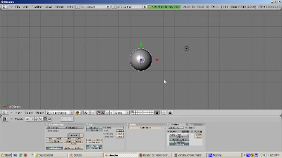
Blender's particle system is flexible and powerful. It can be used for simulating effects like fire, hair, fur, rain. Particles can be emitted from any kind of mesh object. The purpose of this video is to acquaint you with the basic controls for a particle emitter. We'll use the plane, which is the simplest to show. Switch to animation view, with 100 frames.

1) Delete the default cube (Right click, then X, then confirm delete). Add a plane (Space - Add - Mesh - Plane). Subdivide the plane once (W key, then subdivide). Then go to the SR1-Animation view.

2) Go to the Object buttons (F7), then click the Particles button, all the way to the right. We will look at emitter type particles, where the number of particles and their direction change over time. Emitters are good for animating rain and fire, where raindrops and smoke particles move over time. The hair type is for more static simulations, like hair and fur.

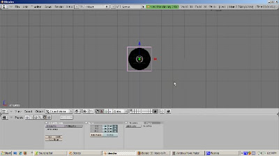
3) Particles are emitted from faces of the plane. The default is 1000 particles over 100 frames = 10 particles per frame.

4) Increase the number of particles to 10000. You see that they're emitting from each face by default. Can change to emit from vertices, as well as volume.

5) Particles are most often emitted from the "normals", the direction that's perpendicular from the face. The Normals setting controls how high the particles are emitted. Set the normal to 1 to show how height is controlled. Press F12 to render.

6) Random adds a bit of randomness to the emitting direction. You can mix normals and random and press F12 to rendeer.

7) AccX, AccY, and AccZ can add an extra push in the respective direction. Set AccX to .5, which gives bias in the X direction of .5 blender units. This is good for fire and smoke effects. Press Alt-A to see the path of the animation.

8) Emitting also works in negative direction. For rain, if you float a plane above the scene, and make it a particle emitter, this would be the start of a rain simulation. You can increase the randomness as well. Set Normals to -.5 and AccX to -.3. Properly textured, this could simulate a heavy rainstorm.

9) Start and End are the start and end frames for the particles. Life is how long the particle lives. Increasing the life makes the particles stay around longer. Start can be negative, which means that the particles are alive at the beginning of the animation.

Increase the life to 100. The particles stay around longer. For fireworks, you might want to vary the life and add some randomness to the emitter.

10) Start can be a negative number also. A negative start number means the simulation began before the first frame is rendered, like the fire is already going at frame 1.

11) Go to a frame 41 and press F12 to render. The particles render as halos, and the plane does not render. The emitter does not render by default.

12) Add a material, F5, shading, make the particles red (R=1, G=0, and B=0). Then press F12 render.

13) To change the halo effects, press the Halo button in the Render Pipeline panel. In the Shaders panel, you can change the halo size. You can also customize the halo - Rings, lines, stars.

Render (F12) for
1) Halo with 4 rings and .5 size.
2) Halo with size .1, 3 stars, and 4 lines

14) Many material settings can be animated. Look at Halo Size. Go to IPO window. Select the Material type curves. Then select HaSize. Create an IPO curve, with Control-Left Click, creating IPO points for size. This creates a Bezier curve for the halo size, which will make them emit with different sizes over time. Here's the resulting video.

These are the basic controls and look for emitter type particles, which work well for fire and rain. We've barely scratched the surface. I hope this gives you a good start towards understanding Blender's partcle system. Happy blending!

2.49b Fluid Simulation

The purpose of this video is to show how the objects in Blender's fluid simulator work. We'll look at domains, obstacles, inflow, outflow, and of course fluid objects. Blender's fluid simulator at first seems very challenging. However, if you think about how fluids behave in real life - think of water pouring out of a faucet into a sink or a bathtub, the fluid simulator starts to become more logical. In this tutorial we're going to focus on the objects in Blender's fluid simulation.

Let's start with the most basic fluid simulation. At a minimum, the fluid simulator needs two things: a fluid, which can be free flowing like a waterfall or muddy like water in a pond; and a domain, which is an area in which the fluid lives. Be warned. This doesn't look exactly like water dripping from a faucet, but it does look like some icky gook falling down in a fluid like manner.

So start Blender. Usually we delete the default cube. This time, however, we will use the default cube. It will be the domain, the area in which the the fluid lives. Go to Front View, by pressing NUM1. The blue Z arrow will point up. We need this because fluids are affected by gravity. In Blender, Z is up and -Z is down.

Let's make the domain a bit higher along the z axis. Press the S key to scale, then the Z key, then scale the cube up 4 blender units. Grab it, with the G key, and move it along the Z direction (Z key) so the domain sits on the X axis. Before we do anything with the cube, duplicate it (Shift-D) and move it away from the original cube. You'll see later why this is a good idea.



Just to track things, let's name our objects. Select the original cube. Press the N key to bring up the Transform Properties window. Rename the cube to Domain. Make sure the cube is in object mode. Press Tab if the cube is in Edit mode.

To tell the fluid simulator that the cube is the domain, press the Object buttons (F7), then the Physics button, the second button in second group of buttons. Press the Fluid button the enable the fluid simulator, on the extreme right. Click the Domain button.



Press the Z key to go into wireframe mode. You can see objects inside of other objects in wireframe mode.

We need to add a fluid. Add an icosphere (Space - Add - Mesh - Icosphere), accepting the default of 2 subdivisions. Scale it down using the S key, so that the icosphere looks like a drop and is positioned at the top part of the cube. Make sure that the icosphere is inside the cube. Check out all the views and rotate, to make sure.

In the Transform Properties window, rename the icosphere from Sphere to Fluid. Let's make the fluid source green, just so we can see it. Press F5 to add a material. To make the fluid source green, set R to 0, G to 1, and B to 0.

Select the domain and go to the material buttons. Make the domain color red by setting R to 1, G to 0, and B to 0. Weird things happen to the domain during the fluid simulation, as you'll see.

To tell fluid simulator that the icosphere is the fluid, make sure the icosphere is in Object mode. Then press the Object buttons (F7) and the Physics button. Press the Fluid button to enable the fluid simulator. Click the Fluid button.



We're set up to run the fluid simulator. The cube is the domain and the icosphere is the fluid. To run it, select the cube. In the fluid simulator buttons for the cube, press the big BAKE button. The cube turns into a blob and starts falling down like a drop. The falling stops where the cube used to be, as if the cube was still there, although it doesn't show.

Believe it or not, we've created a fluid animation. Press Alt-A to see it. Press Esc to stop the animation. The animation is done over 250 frames by default. To create an animation, press F10 (Scene buttons). Set the Output Directory to the directory where you want to store the animation. In the Output panel, navigate to the directory and then select Select Output Pictures. In the Format panel, select the type of video you want to create. The default is jpeg. I like the .avi format, with the CamStudio 1.4 Lossless Codec. I use CamStudio to capture screen shots for these tutorials. If you choose uncompressed the video will take a lot of space. Click the ANIM button and wait. The animation is being created, all 250 frames of it.

Depending on your computer, the animation can take a long time, up to 10 minutes.

I paused the video because it's kind of boring to watch the animation being created frame by frame. Here's the result.



Some things to note. The fluid looks too geometric to be believable. We can help this by smoothing the fluid. Select the domain object, which controls the color of the fluid as it falls. Go to the edit buttons. Press the Set Smooth button. Also, subsurfing the fluid will help. Add a subsurf modifier at Level 2. Select the domain. Press the BAKE button. For the sake of speed, let's reduce the number of frames to 50. At 25 frames per second, this is a 2 second video, but it illustrates the point.

Select the Fluid object. Go to the Physics buttons and change its type from Fluid to Inflow. Here's the result.


The fluid is more, well, fluid-like. An inflow is a fluid object that adds fluid. Blender allows more than one fluid source, i.e. more than one inflow, like more than one faucet or shower head. However, only one domain is allowed.

We're going to add an obstacle. Add a cube below the path of the fluid. Select the cube, making sure it's in Object Mode. Click on the Object buttons, then the Physics buttons. Go to the Fluid simulator. Enable Fluid and click on Obstacle. Running the fluid simulator produces the following result.


Finally, we're going to add an outflow, which takes fluid away from the simulator. An outflow is like a bathtub or faucet drain. To do this, add a plane above the cube, in the path of the fluid. Select the plane, in object mode. Go to the Fluid simulator, as before. Enable Fluid and click the Outflow button. Select the domain and press the Bake button. The animation should look as shown, The fluid disappears before it hits the obstacle.

Remember the cube domain that we duplicated before? To make the simulation realistic, position it on the domain boundaries. You'll need to make it transparent and add materials and textures, no doubt. And probably you will want to apply a realistic water, oil, or mucky texture to your fluids. But that's it. We've done a basic fluid simulation, with a fluid and a domain. We've added an obstacle - in real life, something like a bathtub or sink, as well as an outflow, like a drain. I hope this gives you the basic idea of how it works. Happy Blending.

2.49b Realistic Bouncing Ball

Download the Bouncing Ball blend file





At first glance, one might think that animating a bouncing ball would be easy, a simple matter of moving a sphere and adding location keyframes. Sure, the ball would move. However, it would not bounce realistically. Because of gravity, the ball moves slower at the top than at the bottom. The ball actually is stretched a bit in the middle of the bounce and squashes when it hits the floor. Because of friction, the height of the next bounce is less than the height of the previous bounce. The spin of the ball must be realistic as well.

We're not going to address all these things. The purpose of this tutorial, which is based on the Blender 3D Noob To Pro bouncing ball tutorial, is to show the basics of animating a bouncing ball, including squashing the ball using lattice deformation and how to use IPO curves to bounce the ball a number of times without redoing the first bounce sequence again and again. I used Blender 2.49B.

We'll start by deleting the default cube (Right click, pressing the X key, and confirming the delete). Then add a UV Sphere (Space-Add-Mesh-UVSphere), accepting the default settings of 32 rings and 32 segments. From the editing buttons (F9), press Set Smooth. Then add a subsurf modifier at level 2. This gives us a nice round ball.



Press Num1 to go into Front View. Add a Lattice (Space-Add-Lattice). Press Z to go into wireframe mode. Select the lattice. Scale the lattice so that the UV Sphere is inside of it, with the sides of the lattice touching the sides of the sphere.



To make the lattice control the sphere, select the sphere, then Shift Select the lattice. Press Control-P and choose the Lattice Deform option to make the lattice the parent of the sphere. Select the UV Sphere and press F9. Look at the modifier stack. You should see the phrase "Lattice parent deform" at the top of the stack. This means that the lattice modifier was applied correctly. To test this, select the lattice and scale or move it. The sphere mesh should scale or move as well. We'll use the lattice later to squash the ball. The Make Real button would make the lattice permanently control the ball. We can ignore this button for this simple tutorial.

Now it's time to animate the ball. To do this, switch to Scene SR:1-Animation. This built in scene setup has all the windows we need for animation - the Outline Window, the 3D viewport of course, the IPO window, which we'll use later, and the buttons window.




Position the 3D cursor in the 3D viewport and press Num1 to go to Front View. The blue Z arrow should point upwards. We're going to animate the first bounce over 23 frames, which is about 1 second assuming a standard movie speed of 24 frames per second. Press F10 to go to the Scene buttons, and set the end frame to 23.
It's time to insert key frames. Note that we are animating the lattice, not the ball.

Make sure we're in Frame 1. If not, press Shift-Left Arrow or enter the number 1 in the Frame Number area. We start the animation when the ball is at the top of its bounce. Press the G key, then the Z key, to move the lattice up in the Z direction, about 7 blender units or so, to the top of the bounce.

Press the I key and set a key for LocRotScale. Note how there are now 9 curves in the IPO window, for location, rotation, and scale, in the X, Y, and Z direction. You get 3 curves for each, for X, Y, and Z.

Go to Frame 11. Press the G key, then the Z key. Mgzove the lattice down in the Z direction, to 1 Blender unit above the ground. This is where the ball will be squashed a bit. Press the I key and insert a LocRotScale key.

Go to Frame 13. Leave the Lattice in the same position and insert another LocRotScale key.

Go to Frame 23. Move the Lattice back to its position at Frame 1 by pressing the G key, then the Z key, then moving it back to 7 Blender Units up. In real life, the ball should move back somewhat less than that, because of friction, but for this tutorial, where the ball will just bounce forever, we can ignore this. Press I and insert a LocRotScale key.




We have animated the basic bounce. On Frame 12, we will squash the ball. Go to Frame 12. Place the cursor at the base of the lattice. Set the Pivot point to 3d Cursor. Scale the ball on the Z axis by pressing the S key and then the Z key. Press I to insert a LocRotScale key.



In IPO window, move the Green vertical bar back and forth to scrub the animation. We have now animated both the bounce and the squash. Pressing Alt A will also do the animation of the bounce forever. Press Esc to stop the animation.

The reason the ball bounces forever is that the animation is 23 frames long, exactly as long as the ball bounce. That's a coincidence. To demonstrate this, change the animation length to 250 frames. and press Alt A. Now the ball bounces and just stays there from frame 24 to 250 instead of bouncing. Suppose we want the ball to bounce forever no matter how long the animation. To do that, go to the IPO window. Press A to select all the curves. From the Curve Menu, select Extend Mode and select Cyclic. When you replay the animation, Alt A, the ball bounces for the entire animation.

There's plenty more tweaking that can be done to this basic animation. You can add materials and textures to the ball. You can play with the IPO curves to control how the ball moves, stretches, and contracts. I hope this gets you started. Happy blending.

2.49 UV Unwrapping

Hi. The purpose of this tutorial is to show how to unwrap a globe into two hemispheres. This tutorial is based on the UV Map Basics Tutorial, in the Blender 3D: Noob To Pro wikibook. The URL is in the Youtube notes, as well as at blender3dvideos.blogspot.com, the Web site for my tutorials.

Why do we need this tutorial? The reason: UV Mapping was introduced way back in Blender 2.34 and has been extensively rewritten since then. The user interface, and many terms, have changed over time. As examples, UV Face Select mode disappeared in Blender 2.46, and the term LSCM (Least Squares Conformal Mapping) was used up until then. Now LSCM is simply called Unwrap. Many unwrapping tutorials were based on earlier versions. If you try to follow along in the current version, 2.49b, you can get confused. Hopefully, this video will help to show the steps to successful UV Unwrapping in the version most of us use.

So let's get started. Here's the default scene in Blender 2.49b. Delete the default cube (right click, then press X and confirm the delete). Add an icosphere (Space-Add-Mesh-Icosphere), accepting the default of 2 subdivisions. Scale it 3 times (S 3) to make a large globe. Let's smooth the globe out. From the Editing buttons (F9), press Set Smooth. Then add a subsurf modifier at level 2.

Split the 3d viewport horizontally, by clicking on the border, right click, select Split, positioning the vertical line to where the split should be, and pressing Enter. Make the left window a UV /Image Editor window.

Click on the border of the User Preferences window and drag down to show the user preferences. Click View Name so we can see the view name (Top Ortho). Then click on the border and drag up to free up the area for the 3D view.

Tab into edit mode, and press the A key to deselect all vertices. We're going to make a seam for the UV editor to split the sphere in two parts. To do that, press Num3 to go into side view (right ortho). We're going to box select the vertices at the equator so that when the sphere is unwrapped, the UV unwrap program will know how to split the sphere. So box select (Bkey) the vertices at the equator and press Enter. Press Ctrl-E, which brings up the Edge Specials menu, and select Mark Seam.

Press the A key to deselect the seam and the A key again to select all vertices. Press the U key, which brings up the UV Calculation menu. Select Unwrap. This is actually LSCM Unwrap masquerading under a simpler name. There are many other ways to UV unwrap an object, as you can see. The sphere is unwrapped in the UV/Image Editor window.

The easiest way to actually place the image onto the sphere is to export the unwrapping map to an image editor, such as Photoshop or the Gimp. I use the Gimp, but Photoshop will work just as well. To do this, from the UVs menu item, select Scripts, and choose Save UV Face Layout. Accept the default of 512 x 512 pixel map, which is perfect both for non Game and Game use in Blender, and save the file (it's a Targa image file) in your project directory.

Now open up the Gimp. Here are the steps I found that seemed to work well. First, open up the saved file we just created. Then open up the image to apply to the sphere. You can download the globe hemisphere image, BlueMarble 2001-2002.jpg from the UV tutorial wiki page. Go to the targa file first and find the diameter of the spheres that we need to fit the image to. The diameter is 270 pixels.

Switch to the BlueMarble jpg, the one containing the two globes. Choose the Ellipse Select tool and turn on the Fixed Aspect Ratio check box to make sure that we will do a circle select. Select the left globe. Copy (Control-C) the globe to the clipboard. Switch to the reference file. From the Edit Menu, select Paste As, and choose New Layer. Press Enter to confirm. Click on the Move tool (the one with the cross hairs) and move the globe to the center of the top series of triangles.

From the Layer menu, select Scale. Enter 272. I like to go a pixel a two more than the actual diameter to make sure we don't get any background artifacts included. Press Scale and position the expanded globe over the layout if necessary.

Now go back to the bluemarble jpg and choose the Circle Select tool. First Select None, to deselect the left globe. This time, circle select the right globe. Copy (Control-C) the globe to the clipboard. Switch to the reference file. From the Edit Menu, select Paste As, and choose New Layer. Choose the Move tool and move the globe to the center of the bottom set of triangles. From the Layer Menu, choose Scale, and scale the globe to 272 pixels as well.

Press Control-L to bring up the Layers menu. There are 3 layers, the original reference image and the two globe layers. Deselect the original reference image by clicking on the eye. Close the Layers menu. We now can save our file - we'll make it a jpeg - which will be just the two hemispheres. We'll call it FinalGlobe.jpg. Accept the Flatten Image dialog because that's what we want. Click on Export and accept the defaults.

Now go back to Blender. From the Image menu, open the FinalGlobe jpg. You might need to make some last minute tweaks to eliminate some dark background artifacts. Press the Shading buttons (F5). Add a new material. Click the TexFace button to tell the renderer to use the Unwrapped UVs. Press F12 to render. From here, you might need to add a lamp. If you go into Texture mode you can see the image on the sphere.

That's it. I hope this gives you the basics of UV unwrapping a globe image and gives you some ideas for its use. If you want to create games and need images, this is essential because Blender's game engine requires UV textured images. Happy blending.

Blender Community Toolbar

Hi. I'm Ira Krakow. The purpose of this video is to make you aware of a fantastic resource which I think is an essential tool for any Blender user, from newbie to seasoned professional. It's called the Blender Community Toolbar.

The Toolbar installs in seconds on your browser. There are versions for Internet Explorer, Firefox (the one I use because I like open source), and Safari (the Apple Macintosh browser). I also want to point out some of the links that I have found useful. This is just one person's favorites list, and certainly it's not an exhaustive one. Blender has a large and enthusiastic worldwide following of extremely talented people who volunteer their time and knowledge to enrich the experience of working in Blender for all of us.

So let's start with Kernon Dillon, the author of the Blender Community Toolbar and developer of Blendernewbies.com. First, I want to publicly thank Kernon for all the hard work he's put into blendernewbies. Kernon's clear, precise, and even tempered presentations of even the most difficult Blender topics are a pleasure to watch. Two of my all time favorites are:

A five part tutorial on modeling oven baked pretzels in Blender, which describes just about everything about how to make the pretzels in such a way that you can smell the pretzels baking in the oven.

A three part tutorial on making a magic wand with Blender particles.

I'm not alone as a member of Kernon's fan club. You can read Kernon Dillon, A Blender Community Treasure.

Now we'll do a quick tour of the toolbar. At the extreme left is a button with the Blender icon. Click on that and you'll get to the official Blender Web site, blender.org. This is the place to check out the official Blender news, straight from the source. You can download the latest version (2.49b), learn about Elephant's Dream, Big Buck Bunny, and YoFrankie, the Blender open source movie projects, as well as Durian, the latest Blender open source movie, coming soon to your local computer. You can also access Blender's documentation, the wiki, and catch up on the news from BlenderNation.com, another great place to find out what's going on in the world of Blender.

If you're new to Blender, check out the Blender Basics Video Tutorial link, which gets you to BlenderUnderground.com's excellent 5 Part Blender Basics video tutorial. Blenderunderground.com, lead by Apollos, goes beyond the basics, looking inside the hood to show us how Blender actually operates. The philosophy is that to be efficient in Blender you need to know how Blender works, not just mindlessly pressing keystrokes to get a particular effect. My favorites are:

Part 4, especially the discussion of the outliner. After viewing this, you'll know why you need to create a material before you create a texture, or the difference between an object and its data.

and

Part 5, which has an in depth discussion of lighting, shaders, ray tracing, and other good stuff.

The next button has links to tutorials, from the beginner to the advanced level. One I found very useful is the Introduction to Character Animation. This was part of the Blender Summer of Documentation project. If you can master this tutorial, you will be well on your way to understanding how to animate a character in Blender.

The Extras tab contains many links to Blender resources that should give you many ideas. One link I like is the Blender Open Material Repository. It's a database of over 600 materials, ready for use in your Blender projects.

If you want to extend Blender with Python scripts, you can check out How To Use Python Scripts in Blender, as well as the many Python scripts available for download from the toolbar.

The most fun area of the Community Toolbar is the RSS feeds. You can catch up on news from all sorts of sources. As you can see I have over 400 unread articles. Staying up to date with Blender takes just about a 24 hour, 7 days a week, 365 days a year proposition.

I certainly would follow the articles in Blenderartists.org closely. Blenderartists.org is the most popular site for Blender users, as opposed to Blender.org, which is more geared to Blender developers. The toolbar also includes the feed for Blendernation, just another way to keep up with developments. If you want to see how Blender 2.5 is progressing, follow the Blender Development and the Blender Development Log feeds. And to download the latest version of 2.5, follow the graphicall.org feed. What's nice is that the RSS feeds are updated as soon as new content is added, so you'll always be up to date.

Obviously a short video like this cannot get to all the fantastic resources available from the Blender Community Toolbar. I hope I have encouraged you to download it and see for yourself. Happy Blending!

Bump Map Texture

Hi. Many times, simply mapping an image texture does not highlight the detail of the image enough. Blender's bump map is one of the ways that you can make the images in your scene more exciting and realistic. The goal of this video is to show how bump maps do this. In keeping with the October Halloween mood, we'll start with a jpeg image of pumpkins. These pumpkins, like most, have a lot of deep indentations, and other imperfections. In the 3D world, imperfections are good because they make the scene more realistic. Think of an orange peel. What's more realistic, a peel that's orange everywhere, or one where all the ridges and dimples of the orange show? It's the same with pumpkins.

A bump map is a mathematical calculation of each pixel's height, based on an image. The bump map texture is independent of the underlying mesh. This makes bump mapping far easier than trying to simulate the height effects by adding more geometry to your mesh. Think of adding vertices and faces at every place in an orange peel mesh where you want some height or depth.

OK, let's get started.

1) Delete the default cube, with Right click to select, then X, then Enter to confirm.

2) Add a plane, with Space-Add-Mesh-Plane. Scale it up 10 times (S 10 ENTER).

3) Split the 3D view in half. Make the right half a UV/Image Editor window.

4) In the UV/Image Editor window, from the Image Editor, open the Pumpkins.jpg image. At http://blender3dvideos.blogspot.com, I have a link to the image I used. You can either use that one, or load any image you want. Select the Image and click Open Image.

5) In the 3D window on the left, from the View Menu, select Align View, then Align Active Camera To View, or press Control-NUM0.



6) From the Buttons window, press F10 for the Scene buttons. At the bottom left corner is where you can select where the render output will display. The default is a separate window. Change it to Image Editor. This will let us compare the reference image with the image with our adjustments applied.




7) Select the plane (right click). Add a material, by pressing F5 (Shading), then the Material purple sphere, then click Add New.

8) We're going to select a color from our reference image as our base color. Later, we'll change it to see different effects. Click the Color rectangle, then the Sample button. Go to the reference image in the UV/Image Editor window, and select an orange color that will serve as the background color for the rendered image.



9) Press F12 to render. The plane is orange, but there's a big white spot on the upper right corner of it. This is the result of specular highlights. We want to turn this off. Click on the Shaders tab, find the Spec slider, and turn it to 0. Press F12 to render. Now the specular highlights are gone.



10) Press F6 for the texture buttons. Click Add New. Click on Image. Select Image as the Texture Type. Click on the Load button. Load the Pumpkins.jpg image. Press F12 to render. The pumpkin jpeg is now on the plane.



11) To make the image a bump map, click on the Material buttons. Go to the Map To panel, all the way on the right. We'll make a full bump map. Turn off Col, for Color, and turn on Nor, for Normal. Increase the Normal slider to 20, to make the effect obvious. Press F12 to render. As you can see, the pumpkins look more realistic than before, but we don't have any color.



12) Turn on the Col button, and press F12. Now the orange pumpkin color is back without affecting the bump map.



There are many other artistic type effects you can do. Here's an example. Go to the Texture buttons, F6. Change XRepeat to 4 and YRepeat to 4. This makes the image repeat. The bump map effect repeats as well.



Any time you want to save a render, press F3. You can use the JPEG somewhere else, say as part of a Halloween party invitation. I think you'll agree that this is much easier than creating a mesh that looks like these pumpkins. I hope this gives you some ideas about how to use bump maps to make your Blender scenes more realistic.

Radiosity Rendering

Download the blend file



Hi. Conventional lighting systems use lamps and cameras. The light is emitted from the lamps, bounces off the object, and then interacts with the camera to determine how the object is lit. The object is basically a passive receiver of light.

Radiosity takes a different approach. No lamps are necessary, although radiosity can be used to supplement traditional lamp based lighting. Instead, the objects themselves, or at least the ones you designate as light emitters, are the light source. They also receive light, but this time from other objects. This occurs in real life, and it's not limited to lamps. Think of lit matches, fire, glowing embers, or atomic bombs. Radiosity is a mathematical calculation of how objects that emit light interact with objects that receive light. Most objects actually do both at the same time. Radiosity rendering can produce stunning effects, but it takes getting used to. The goal of this tutorial is just to make you comfortable with radiosity setup.

Start by deleting the lamp. Radiosity does not need the lamp because the light comes from the materials applied to the objects. Right click on the lamp, and press X to confirm the delete.

Add a UV Sphere to the scene, with Space-Add-Mesh-UVSphere. We'll give the UVSphere 16 segments and 16 rings. The top half of the UV Sphere will be our light source, acting somewhat like a hemi lamp, with a soft hemispheric lighting effect and soft shadows. Move the UVSphere so that it is above the cube. Grab it, with the G key, and move it up. Scale the UVSphere 5 times - S 5 then ENTER. Press Z to go into wireframe mode and Tab to go into Edit mode.

We need to delete the bottom half. Press the A key to deselect the vertices. Then box select (B key) all the bottom vertices. Press the X key to delete the selected faces on the bottom half. We're left with a hemisphere.

Press F5 for the Shading buttons, and click on the Material button. Click Add New to add a material. Give the cube R, G, and B values each of .5, so that the hemisphere will emit equal amounts of each. Click on the Shaders panel, and set the Emit value to .02. It's a small number, but the UVSphere has many faces which will generate sufficient light for the scene.

We need to make sure that the normals are pointing towards the cube. Light is emitted from the face normals. Press F9 to go to the Edit buttons. In the Mesh Tools More panel, click on Draw Normals. Set NSize to 1.0. Select all the vertices by pressing the A key. Note that the normals are outside, so the light will not reach the cube. To fix this, press the W key and select Flip Normals to have the face normals point inward.

Before we continue, we need to make sure radiosity is enabled in our render. Press F10 for the Scene buttons, turn on Radiosity, and turn off SS, Ray, Shadow, and Envmap. The entire scene will be lit by the UVSphere radiosity.

Let's set the camera as well. Set the scene so that the UVSphere is providing hemispherical light to the cube, which is a bit off of the plane. Move the hemisphere up a bit, out of the camera view. Move the camera in a bit towards the cube.

Now we'll create a white ground plane from which the shadows will fall. Tab out of Edit mode. Add a plane - Space-Add-Mesh-Plane, and scale it 5 times - S 5 Enter. Grab it and move it below the cube with some space between the bottom of the cube and the plane.

Press the Shading button (F5) and add a new material by clicking the Add New button. Make the plane white by setting the R, G, and B sliders all the way to 1. We need to make sure that the normals are facing upward. Tab into Edit mode. In the Editing Context, Mesh Tools More panel, click Draw Normals and set Normal Size to 1. The normals point downward. They need to point upward. Press the W key and select Flip Normals to fix this.

Tab out of Edit mode. Select the cube, Shift F2. Click the Shading button, F5. Set the material color to Blue, R=0, G=0, B=1. Tab into Edit Mode. We need to check the normals. From the Mesh Tools More panel, click Draw Normals and Set Normal Size to 1. Indeed, the normals face outside, which is correct. Tab out of Edit mode.

Now we're ready for our first radiosity render. Tab out of edit mode. Press the Radioactive icon, for radiosity. Before we start the calculation, press the Gour button, which is a good choice for radiosity with shadows. Shift-Select the cube, the plane, and the UV Sphere: every object in the scene except the camera. All of these will participate in the radiosity calculation. In the Radio Tools panel, click the Collect Meshes button. Now we're ready for the calculation. Click the big GO button for the radiosity calculation. I'll pause the video while the radiosity calculation does its thing. See you when it's done. Press F12 to render.

Next, we'll add a yellow monkey next to the cube. First, press the Free Radio Data button to clear the radiosity calculations. We are going to recalculate te radiosity after we add the monkey. Press Space, Add, Mesh, Monkey. Click the Shading Buttons, F5. Add a yellow material, by clicking the Add New, and setting Red to 1, Green=1, and Blue to 0. Note that Ambient is .5, which means that the monkey can receive 1/2 of the light sent to it from the UVSphere. Emit is 0. The monkey is only receiving light, not emitting it. Tab into Edit mode. Press F9 for the Edit windows. Note that the face normals are pointing outward, to receive the light, so we're fine.

Tab into object mode. Smooth the monkey by pressing the Set Smooth button. Then add a Subsurf modifier at Level 2.

Press F12 to render. I'll pause the video again until it's done.

This just scratches the surface. You get more realistic rendering if you work with more geometry. Experiment with the different settings that influence the radiosity calculation. You may want more defined shadows or a different color mix. You can also mix radiosity with other non-lamp lighting effects, such as ambient occlusion. Happy Blending!

Halloween Mask

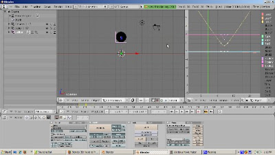
Modeling with curves is a powerful Blender feature. Few objects in life are pure straight lines. Life continues to throw curves at us. As an example, we're going to make a Halloween mask with Bezier curves.

Blender itself uses Bezier curves extensively. The curves in the IPO window, as an example, are Bezier curves. So if you're going to be animating your scene, you can do a lot more if you understand how to manipulate Bezier curves. There are also some great modeling tools, such as loft modeling and beveling, which rely on Bezier curves. Knowing how to deal with Bezier curves is a fundamental Blender skill.

Start with the default Blender scene and delete the default cube by right clicking it, pressing the delete key, and confirming the delete. We'll work first with a special case of the Bezier curve, the Bezier circle. A Bezier circle is a Bezier curve that just happens to be a circle as well. Like all Bezier curves, and also like mesh objects, the Bezier circle can be moved, scaled, and rotated.

How does the Bezier circle differ from the mesh circle? A mesh circle is defined with a certain number of vertices. The more vertices, the closer the circle looks like a circle. Of course, it's never a perfect circle. You pay a price for more geometry in terms of rendering time and modeling complexity.

A Bezier circle is a true circle, as opposed to a circle mesh, which never can be an exact circle because it's composed of straight edges. We can increase the number of vertices, do smoothing, and other tricks to make it render close to a circle, but it's never an exact circle. Also, mesh circles have modeling problems such as dark edges where normals are inside the mesh, instead of outside the mesh, where the edge can render with light.

Delete the Bezier circle. We'll look at the more general case of Bezier curves. Our goal is to create a mask using Bezier curves, and then to convert it to a mesh.

Start with adding the Bezier curve, with Space-Add-Curve-Bezier Curve. A Bezier curve is a curved line called a spline. At either end are control vertices, which you can select, grab, and move around. In addition to the control vertices, one at either end, there are lines that extend out, which are called control handles. You can select a handle, move it in or out. You control the shape of the curve by controlling the handle. The handle on the left controls the shape of the spline coming in. The handle on the right controls the shape of the spline coming out.

You can add vertices by pressing the Control key while left clicking with your mouse. We'll add a few vertices to start the face. The handles on either side of the control vertices are purple lines. The handles by default are align handles. The other handle aligns with the one you select. You can change from Align to Free by pressing the H key. The handles turn black and you can turn each one individually. One handle controls how the curve moves into the control vertex, the other controls how the curve move out of the control vertex.

For creating a simple outline, the easiest choice is Auto, which you turn on with Shift-H. Auto automatically smooths out the curve coming in and out of the spline. So we'll turn on Auto with Shift H.

Control-Left Click creates an additional control vertex, so you can make a shape from an outline. We'll make the face part of the mask first. Then we'll cut out the eyes and the mouth. We'll add more splines to the curve. You can use the handles to control the shape of the curve. You can select a vertex, in which case the handles are selected as well. You can control the curve path through the handles as well.

When you're done with the outline, and you want to close the curve, select a vertex and press the C key. The curve then closes.

You can create straight line handles easily. Select two adjacent vertices and press the V key. V is for Vector. This makes the curve become a straight line. Press Ctrl-Z to undo this because our mask doesn't have straight lines. Frequently, you will have to model an object, such as a wineglass, that is a mixture of straight lines and curves.

You can still edit the face and add more depth to it.

By default, you control the curve in 2D space. You can't move it in 3D space unless you go to the Curve and Surfaces panel and switch on the 3D button. Then you can grab one of the control vertices and move it in 3D space.

We can also make the mask 3D. Turn on the 3D button and you will see perpendicular lines, like a porcupine, jutting out of the curve. You can extend the curve into 3D if you want.

Now we'll add two eyes, which will be Bezier circles. Do Space-Add-Curve-Bezier Circle. Scale down the circle and press the G key to move it to where the left eye should be. Note that there's a hole cut out of the face for the eye. Press Shift-D to duplicate the circle. Press the G key and position the second circle to where the right eye should be.

Let's make the mouth using another Bezier curve. Do Space, Add-Curve-Bezier Curve. Press Shift-H to go into Auto mode. Add vertices - CTRL-Left Click - until the shape of the mouth looks right. Then press C to close the curve. Select the vertices of the inner circle, press the S key to scale the mouth. Go into object mode.

The Bezier patch is 2D. Let's extrude the mask to give it some depth. As you increase the Extrude value, the mask gets thicker. You can also bevel the mask to round out the edges. The mask can still be edited as you go.

It's time to turn our mask into a mesh object. To do this, tab out of edit mode, and to convert it, do Alt-C to convert to a mesh. From there, all the mesh functions are available. We'll smooth it and add a subsurf modifier. We can do a lot more, in fact, such as changing to face mode and extruding some faces to create a nose, or grabbing some faces and moving them.

To sum up, working with curves is a powerful addition to your modeling arsenal. If you can visualize your object from a curved outline, using curves, including Bezier curves, is a powerful way to create a Blender object from your outline.