2.53 Beta Add Ons

It's so new that the URL still says alpha! Versions of 2.53 Beta can be downloaded for Windows 32bit, Windows 64 bit, Linux 32bit and 64 bit, Mac OS X, and Solaris. As a beta version, the basic features should be in place, although bugs are still expected. There are many bug fixes, some reorganization of window choices, and some new features. You can read more about all the changes in Blender 2.5, at:

http://www.blender.org/development/release-logs/blender-250/

In this tutorial, I'm going to talk about the new Add-On repository, which is a way to extend Blender functionality by adding Python scripts. A number of these scripts are shipped with 2.53 beta. They are documented online in the Blender 2.5 Add-Ons Repository, at:

http://wiki.blender.org/index.php/Extensions:2.5/Py/Scripts

I will show you where the add-on scripts are stored and how to install and run them. I will also show you how to edit the source code of the installed scripts, which are a great resource for learning how to write add-ons.

Blender 3D Cookbook, Volume 1

I am pleased to announce the publication of Volume 1 of my Blender 3D Cookbook available from lulu.com, either as a book or a PDF download, at:

http://www.lulu.com/product/paperback/the-blender-3d-cookbook-volume-1/11777448

The Blender 3D Cookbook consists of the scripts to 62 or my my Blender 3D tutorials, at http://www.youtube.com/irakrakow. Each script has a link to the Youtube video, if you purchase the book as a PDF. If you purchase the book, the URL is printed. Many of you have requested such a book. I called the book a “cookbook” because you can think of the scripts as “recipes” for producing a desired effect in Blender.

I don't assume any particular level of Blender expertise. My videos cover a wide variety of topics, from beginner to advanced, including some that I have not seen as tutorials anywhere else. Like a cookbook, you can pick and choose those recipes you are interested in and skip the ones that you either know about or that you're not interested in. I tried to include something for everyone, including topics such as the Blender Game Engine and Python scripting that have only been lightly covered in other tutorials. If you have suggestions for future tutorials, please email me at ira.krakow@gmail.com.

As of this date, Blender is undergoing a massive rewrite and restructuring. The current, production version, 2.49b, will eventually be replaced by version 2.5. 2.5 has a different user interface and has many improvements to old features, as well as many new features. It is currently in alpha, which means that there could be some changes made until the day when 2.5 becomes the production version of Blender. On my Blender 3D forum, at http://forum.irakrakow.com, I took a survey of who used what version. I discovered that roughly half worked in Blender 2.4x (although 2.49b is the most current production version, some were working in earlier versions), and the other half worked in Blender 2.5. I have written tutorials based on both versions. For each tutorial, I note which version (2.49 or 2.5) I made it for. Some of the 2.5 tutorials were done in different alpha versions, such as Alpha 0 or even pre Alpha. For the most part, the effects I write about can be produced in any version.

These tutorials are not intended to cover every conceivable Blender feature. That would, in my opinion, be too thick a volume. Note that I suffixed the title to this cookbook “Volume 1”. Blender is too complex and rich a program, undergoing constant upgrading and changing, for that. I plan on publishing many more volumes of the Blender 3D Cookbook, in the future, that will explore other amazing and unique Blender features.

I welcome your feedback and hope you enjoy my cookbook.

2.5 Empty Object

The name of this video tutorial is Empty Object. A big Thank You to Neal Hirsig (nhirsig@tufts.edu), who created the tutorial on which this tutorial is based, at http://www.gryllus.net. An Empty Object is a non renderable object that represents a point in space.

2.5 Splitting and Joining Windows

The name of this video is Splitting, Joining, and Expanding Editor Windows. It is possible to expand an editor window by moving the cursor to the edge of the window until you see a double arrow. Left click and drag the window open. This can be done horizontally or vertically.

Free Blender Render Farms

Join my Blender 3D forum where you can network with other Blender friends and get your Blender 3D questions answered.



One of the most significant challenges for Blender users is that, when scenes become complex, with meshes containing many thousands, or even millions, of polygons, complicated physics, many texture and material channels, many render layer passes, all of which are animated, render times on even a powerful PC can become unacceptably high. These can stretch into even days or weeks. You might think that you would need a Pixar-size budget to get acceptable render times. In fact, it's possible to significantly reduce render times, I mean by factors of 10 or 100, for free. The answer is to use one of the free render farm options available. I believe that Blender, combined with using one of these render farm options, can help you to approach Pixar-like, or Avatar-like, quality videos with a fraction of Pixar's budget, or even with no budget at all. That's why I call Blender "Pixar on your laptop". I hope Pixar doesn't sue me for this slogan. My goal for this video is to show you how to either create your own render farm if you have some spare PCs hanging around, and you have a wireless Internet connection, or how you can use one of the free, open source, to grab the computer power you need.

First, here's a quick and dirty way to create a render farm with some spare PCs that you have networked. The only real requirement is that you have enabled file sharing on, say, a Public folder in your network. I don't know what operating system - Windows XP, Vista, System 7, Linux, Mac OS X, whatever - that you're working on, but I'll assume that you have some way to share files. Once you've done that, create the Blend file that you want to render. Press the Scene button (F10) and in the Output directory, enter the name of the shared folder (I entered /IRA-PC/Public just as an example). Then press the Touch and the No Overwrite buttons. What this does is allow any temporary files to stay around. Save the file. Then copy the Blend file to the Public folder, making sure the file is shareable. The last step is to go to each PC on your network, open up the blend file, and press the ANIM button. Each computer will then start up at the next unrendered frame, thus sharing the rendering load. Try it. Tell us your results by going to my blog for these tutorials, at http://blender3dvideos.blogspot.com, and adding a comment.

OK, now suppose you don't have spare PCs available and want to speed up your renders like the big guys. No problem. There are a number of free, open source, render options available. I'll show you two of them. The most commonly used one is FarmerJoe, which you can download at www.farmerjoe.info (Make sure you use the .info suffix.) I haven't installed it, but I did download the zip file. The install appears to be simple enough. Unzip the file, in Windows, run the exe file, and then run the Python script to schedule jobs. There's a Web app server to check the status of your job. Again, try it and tell us your results by adding a comment to my blog at http://blender3dvideos.blogspot.com. I'll post the full URL of the blog page on the Youtube notes to this video.

Another possibility is the University of California, Berkeley's BOINC project, which uses the spare computer cycles of PCs around the world, available for anyone to share. You can join the network, at http://boinc.berkeley.edu and trade your idle CPU cycles with other PCs. There's plenty of idle computer time to go around. Why not make use of it?

Maybe you have other ideas? If so, please share them by commenting, either on my blog at http://blender3dvideos.blogspot.com, or leave a comment on this video. If you liked this, remember to hit the Youtube Subcribe button so you won't miss any of my future Blender tutorials. Happy Blendering!

2.49 Armature Animation

Join my Blender 3D forum where you can network with other Blender friends and get your Blender 3D questions answered.

Download the blend file



The purpose of this video is to show how armature animation works in Blender 2.49b. Understanding how to move the bones in an armature is the key to being able to rig a character. We'll first create a basic skeleton-like armature. Then, I will show the difference between FK (Forward Kinematics) and IK (Inverse Kinematics). I like IK in particular because my initials are IK. It's also something we both have in common with the exquisitely unreadable German philosopher, Immanuel Kant.

Leaving the Categorical Imperative aside, we will create a simple hand wave cycle and introduce the Action Editor and the Non Linear Action Editor (NLA Editor), to give you an idea of how actions are defined and how they can be layered together to produce complex movement. We're concentrating on the armature only, how the skeleton moves, so to speak, not the object to be rigged. Once you have an armature, say, of a human, moving correctly, you can then rig it to a human-like object. This is the theory behind the ManCandy rig. I will discuss skinning, the process of associating an armature with a character, either 2 or 4 footed, or I guess any-other-number-of-footed creature, in another tutorial.

Steps:

1) Delete the default cube. We're going to create a primitive skeleton. Go to Animation view by selecting it from the View dropdown. Go to Front View (Num1). Add an armature (Space - Add - Armature). Scale the bone up 4 times (S - 4 - Enter). Look at the Outliner. Expand the Armature outline. Note that the Armature has one bone, called Bone.

Tab into Edit mode. A bone is a child object to the armature. A bone has three parts, the tip, the root, and the body. A bone can be selected in one of two ways. One way is to select the bone's body, which will also select the bone's tip and root. The other way is to right click on the body and shift right click on the root, which selects the body, which is between the tip and the root. Press W for the Specials menu. Select Subdivide Multi, with 4 cuts. So now we have 5 bones, which can function as a primitive spinal cord. Expanding the Armature display in the outliner shows that the bones are named Bone.001, Bone.002, Bone.003, and Bone.004, parented to Bone. You can also see the names in the 3D view by going to the Edit buttons (F9)and pressing the Names button. Press the Names button again to turn the names off.

2) Turn on X-Axis Mirror. This is a handy tool which lets you create mirrored bones on the X axis. When the bones are symmetrical, using X axis mirror means that you only need to create bones on one side. Mirrored bones are created on the other side. Normally, to simply add a bone, you press the E key, which extrudes the bone. However, with X-axis mirror turned on, you can add mirrored bones by pressing Shift-E. If X-Axis Mirror is turned off, Shift-E acts like the E key, just extruding one bone. we'll also mirror extrude 2 legs with Shift-E.

Here's how it works. We're going to create two primitive arm bones, on the left and the right, at the same time. With the tip of the 4th bone of the "spine" selected, press Shift-E. This creates two bones, on the left and the right, which can be scaled. Press Enter when the bones are at the desired size. Select the tip of the newly created bone on the right and press Shift-E again. This creates two more mirrored bones.

We can create mirrored legs. Select the root of the lowest bone of the armature. Press Shift-E to create two "legs". Then select the tip of the bone on the lower right. Press Shift-E to create two more bones, for the feet. I hope you get the idea. I'll leave it to you to create fingers and hands, but for now, we have the basic skeletal bone strucure.

Let's see how bones are named. From the Editing buttons, in the Armature panel, click on Names. Names shows you the names of the bones that were generated. An easy way to see how the bones are named is by using the Outliner. The original bone is called Bone. The spine bones were created with the suffix .001, .002, .003, when the big bone was subdivided. Mirrored bones, the ones created with Shift-E, have an additional _R and _L, depending on whether they are created on the left or the right. Look at the outliner. You can see that each leg is parented off the base bone, Bone. If you look at a detailed armature, such as the Mancandy rig, you'll see that the bones have meaningful names, like Left Arm, Right Pinky, and so on.

The outliner clearly shows parent-child relationships in the armature. This is important when we start posing the armature. Turn off names.

3) OK. Now we have a basic skeleton. Let's see how the bones move, in particular the difference between forward kinematics (FK) and Inverse Kinematics (IK). Blender has a special mode, called Pose Mode, allowing us to move bones so that the armature ends up in the position we want. We're going to create a simple arm wave, what Blender calls an Action. Blender has a special mode, called Pose Mode, for moving armature bones. We're at Frame 1. Select the two bones for the right arm (Right click on the arm, then Shift-Right click on the second bone). Press the I key. Select LocRot.

The curves don't appear in the IPO Curves editor, although they were created. The reason you don't see the curves is that you need to go to the Pose curves. Change the curve type from Object to Pose.

A handy feature in the timeline is the red button that automatically records keyframes as you move bones around. If you don't press it, you would need to remember which bones you moved as you keyframe. This way, Blender keyframes each move as you do it.

Now go to Frame 11 by pressing Up arrow or entering the number 11 in the current frame area. Select the arm bone and press the G key to move it up a bit. Then select the other arm bone and press the G key to move it up in a salute type position.

We've actually created half of the waving action. We'll complete it now. Switch the window from the IPO editor to the Action Editor. Note that there are 2 keyframed bones, Bone.003_L, and Bone.003_L.001. The diamonds indicate the keyframe. To complete the wave, select the two diamonds (they're yellow when selected and white when unselected), at Frame 1. Then press Shift-D to copy. Finally, drag the two diamonds to Frame 21. Drag the vertical green arrow and watch the wave. Press Control-DownArrow to maximize the Action Editor. Rename the action to Wave, from Action. Press Control-DownArrow to return the Action Editor to it's original position.

Let's see the difference between FK and IK. Select the right arm bone. Turn on the AutoIK button. Grab the arm and move it. Note how the whole skeleton, except for the legs, move. This is definitely not how an arm moves. It's actually more appropriate for a leg. IK actually does movement backwards, to the root of the skeleton. You can change how far back the IK calculates by disconnecting a bone. To show this, select the third bone, go into Edit Mode (Tab), and click the CON button, which disconnects this bone. Go back into Pose Mode. Select the arm again, and move it. Note that the movement stops at the disconnected bone. FK does movement forwards.

There's one last window to see, the NLA Editor. This lets us mix different types of actions. Change the window type to NLA Editor. You should see the Wave action. If you press the C key while the Wave action is highlighted, you're prompted to change the action to an NLA Strip. Press Enter. These strips can be combined (wave + walk + hip swivel + talk, and so on). A detailed explanation of the NLA Editor is the subject of a future tutorial.

So that's a brief look into the basics of animating an armature. I hope you enjoyed it. If you did, be sure to hit the Youtube Subscribe button so you won't miss any of my future tutorials. Happy Blendering!

2.50 Animation Part 2

Join my Blender 3D forum where you can network with other Blender friends and get your Blender 3D questions answered.

Download the Blend file



In my first animation video, I showed how to keyframe location, rotation, scale, and material color, as well as how to group keyframed properties into keying sets. I left you probably wondering how, considering that the IPO window has disappeared, you can change the curves by editing them as you could do in Version 2.4x. In this video, I will show you how this is done, and how, overall, the animation process is easier than before. We will also look at some properties that now can be keyframed, such as modifiers, as well as the new F-Curve system.

Steps:

1) Start with the default scene, with the default cube. Change to the Animation view. In the Animation view, there are a number of new windows, in addition to the 3D window. The three that specifically relate to animation are on the left part of the screen. At the top is the Dopsheet, which is the new name for the Action Editor. As before, pressing Ctrl-down arrow makes the window full screen. We'll be doing this a lot in this video, to see what's going on in a particular window. Pressing Control-down arrow again returns the window to its original size.

In the middle left part is the Graph Editor, which is the new version of the 2.4x IPO Editor. You can edit animation curves in the Graph Editor. The organization of the curves has been redone, with major enhancements which I'll point out as we go.

At the bottom right corner is the timeline, the window which has changed the least. As before, you can scrub the animation by dragging the vertical green arrow, and the VCR llke keys do roughly what they did before. As I mentioned in the 2.50 Animation Part 1 tutorial, you can now run the animation backwards.

Before we start, set the end frame of the animation to 50 frames by entering 50 in the End area of the Timeline.

We're going to insert a LocRotScale keyframe at Frame 1, to start the animation process. It works the same way. Position the cursor over the 3D window. Press the I key. Select LocRotScale. Let's see what happened. It looks like there were some curves added in the Graph Editor. Press Ctrl-Down Arrow to see what was added. We can't see what curves were added until we click on the left arrow, to expand the display.

Nine curves indeed were added, location, rotation, and scale, in the X, Y, and Z direction, as in 2.4x. The rotation curve has a new term - Euler - that wasn't there before. That's because rotation can be done in what's called Quaternions, as well as Eulers. For the time being, ignore this. Eulers are what we know as XYZ. We'll go into more detail about these curves after we actually animate the cube.

Press Control-Down Arrow to return the Graph Editor back to its original size.

Go to Frame 25. Press the G key and drag to move the cube over 4 or 5 Blender Units. Press Enter when done. Scale the cube up 2 times (S - 2 - Enter). Rotate the cube 45 degrees (R - 45 - Enter). Press the I key and insert an LoRotScale keyframe. Let's see what happened in the various graphs.

Start with the Graph Editor. Indeed, there are now 9 curves that we can see. They're all visible because all the check boxes at the left are checked. There's also an individual color assigned to each curve, such as red for the cube's X location. Let's in fact edit the curve for the cube's X location. To do that, uncheck all the boxes except for the X location curve. As before, each curve (they're now called F-curves) is a Bezier curve. You're in edit mode, with all the points, each representing a keyframe, selected. Press A to deselect all. Then right click on the ending keyframe. Move it up 2 Blender units or so by pressing the G key and moving it up. If you uncheck the Cube group and then check it again, all the curves display.

The lock icon controls whether or not a particular curve can be edited. If you click on it, the lock icon goes into the locked position and it can't be edited. If you click on it again, the curve is unlocked and can be edited.

Press Ctrl-Down Arrow to return the Graph Editor to its original location.

Press Alt-A to run the animation. The cube goes in the X direction, according to how you edited it.

The eye icon controls whether or not that particular curve contributes to the animation. It's a toggle. When the curve contributes to the animation, you see an eye. When it doesn't, the icon is greyed out. To show you how it works, click on all the eyes except the one associated with the X location curve. Press Control-Down Arrow to return the Graph Editor back to its original location. Press Alt-A or use the VCR keys to animate. Now the cube just moves in the X direction.

While we were animating, note that the Dopesheet, the graph at the top right part of the screen, was populated. Position the cursor over the Dopesheet and press Control-Down Arrow. These are actions that can be combined in the NLA editor. We won't discuss these in this video. I just wanted to point this out. There still seem to be some problems with screen refreshing of this window.

Let's see what happens when we animate another object. Let's add Suzanne to the scene (Shift-A, Add, Mesh, Monkey). Let's insert a LocRotScale keyframe for her. Press the I key, then select LocRotScale. Some more curves were added. Amazingly, we can edit the curves of both objects. What happened? First, Suzanne is now called "Mesh". There's an object called Mesh, as well as a mesh called "Mesh". As with the cube, the curves for what we used to know as Suzanne are in the Mesh's mesh. If you expand the Mesh Mesh, you'll see them. You can also view the Cube's curves.

Press Alt-Down Arrow to return the Graph Editor back to its original position.

The last thing I'll show in this video is that modifiers can be keyframed. This can make for amazing effects. Let's add an Array Modifier to the monkey. Set the current frame to 1. Then, click on the Modifier icon in the Mesh's Properties. Select Array. Change the count to 4. With the cursor on Count, in the Array Modifier area, right click. Select Insert Keyframe. Then go to Frame 25. Change the count to 2. With the cursor on Count, select Insert Keyframe. Press Alt-A to run the animation. Note how the number of monkeys changed.

Look at the Graph Editor. A new curve, called Count(Array) was created. There also is a Count(Array) curve created in the Dopesheet.

The goal is that any property you can see can be animated. Think of all the modifiers and all their properties that you can now animate easily.

Believe it or not, this only scratches the surface. I hope this tutorial gets you to think about how to use Blender 2.5's animation in your scenes. Don't forget to subscribe to my videos on Youtube so you won't miss any. Happy Blendering!

UV Image Editing

Join my Blender 3D forum, where you can network with other Blender friends and get your Blender 3D questions answered.



The purpose of this video is to show how to edit an image in the UV / Image Editor in Blender 2.49b. Editing an image with the UV / Image Editor is important when you're combining (the technical word is "compositing") images and objects into a final render, as well as for creating custom textures. The process involves mapping a 3D surface onto one or many 2D images, a process called UV unwrapping a mesh. The mapping is done on each face. It's possible for each mesh face to have its own image mapped to it. We'll start with the simplest case of UV unwrapping, unwrapping an image onto a plane, which has, of course, only one face. We'll work our way up from there.

1) Erase the default cube (right click on the cube, then press the Delete key, then Enter). Add a plane (Space - Add - Mesh - Plane). Scale it up 3 times (S - 3 - Enter). Split the window horizontally by right clicking on the 3D Window bottom border, choosing Split Area, and positioning the double arrows so that the window is split.

2) We're going to play with a picture of me, in front of one of the 26 palaces of the King of Morocco, in Rabat, Morocco, projected onto a plane. It's good to be the king. Select the plane. Tab into Edit Mode. Press the A key twice to make sure that all the vertices are selected. Press the U key to unwrap the plane. Choose the default Unwrap method. The result: after you unwrap the plane, in the UV / Image Editor you should see a square with 4 vertices - actually, it's a face.

3) The next step is to load my image. From the UV / Image Editor, select Image, then Open. Select the Image. You might need to use the Zoom In and Zoom Out keys (Num+ or Num-) to position the image so that it fills up the square. There's the picture. In the background are soldiers, in their typical position before the Morrocan Changing Of The Guard.

4) The next step is to get my picture to display, both on the plane in the 3D view, and in rendering the image. We want the camera to see the image projected on a flat plane. To do that, from the View menu, press Align View, then Align Active Camera to View, or press Ctrl - Alt - Num0. Press F12 to render. The plane renders right now with the default gray material.

5) To get my picture to render, we need to tell the renderer to use the texture face (TexFace), which is the image from the UV / Image Editor. To do that, go to the Shading buttons (F5), select the default material (Material). Then, turn on the TexFace button. Now Press F12 to render. A bit better, but the image is upside down. We'll fix this shortly.

6) To see my image on the plane, go to View Properties. Turn on the SolidTex button. If the image still doesn't display, make sure the 3D View is in Solid mode. Now you can see me, upside down, as in the render. How can we fix this? In one of two ways...either by rotating the image in the 3D view or rotating the image in the UV / Image Editor. We're not going to change the geometry in the 3D view. We'll fix it in the UV / Image Editor. To do that, with all the vertices selected, press the R key, then rotate it 180 degrees. You can hold the control key down when you're close to 180 (you can see the rotation at the bottom of the UV / Image editor). That way you get exactly 180 degrees.
Press Enter and the image is now correct, both in the 3D view and the UV / Image Editor.

7) The entire image doesn't have to be mapped to the plane. To show that, go to the UV / Image Editor, with all the vertices selected. Press the S key to scale. Reduce the square to a rectangle syhowing only part of the image. I'm scaling the square down to a rectangle which focuses more on me than on the palace. The square is now a tall rectangle. Press F12 to render. Gee, I gained some weight. Moroccan food can be fattening, I guess.

8) The reason for the weird result is that, although the plane starts out mapped to a square area on the image, when I scaled it down, it became wrapped to the rectangle. The rendering stretched my stomach out, to fill in the plane's square area. That is the problem with UV unwrapping. Each face is mapped in its own way to an area of the image. The way that you unwrap a mesh makes a big difference. I'm going to show you how it can get even more weird. Press Ctrl-Z to undo the edit. That's the fastest diet on record.

9) We can do much finer edits, simply by adding more faces to the plane. To do this, position the cursor inside the 3D view. Press the W key to bring up the Specials menu. Select Subdivide Multi. Make the number of cuts 5. Of course, it can be any number you want. This gives us a 6 x 6 grid, with 36 faces in total. Go into Face Select mode by clicking on the triangle icon. Press the A key to deselect everything. Select a face in the 3D view. In the UV / Image editor, you see both the loaded image, and the part of the image that is mapped to that particular face.

10) Let's see what those guards are really doing. Easy enough. Select the faces that map to the part of the image where the guards are. Press the S key to scale them up a bit. Press F12 to render. They have really neat uniforms, don't they?

11) We can also edit from the UV / Image Editor. Position the 3D cursor in the UV / Image Editor. Box Select the area mapped to my shoulder. Press the R key to rotate it a bit. Now I'm bending my body in a strange way. Press F12 to render.

12) To show you why the projection method makes a difference, I'm going to unwrap the plane based on the Sphere from View projection. The result is as if both me and the King's palace were put through a blender which, in a sense they were. Thank God for Ctrl-Z.

You should play with all the different projection methods in Blender. A cube projection of an image actually will work fine. You can unwrap it and then scale the UV squares to fit the image. You can unwrap as many times as you like. Each unwrap undoes the previous one. However, you can have multiple unwraps if you want. The way to do that is to create a new texture map. The default name is UVTex. Click New and unwrap - the default name is UVTex.001, which you can change - and you can experiment with different unwrappings.

I hope this gives you a start in using the UV / Image Editor. Be sure to hit the Youtube Subscribe button so you won't miss any of my tutorials. Happy Blendering.

Mix Node Part 1

Join my Blender 3D forum, where you can network with other Blender friends and get your Blender 3D questions answered.



One of the powerful reasons for using Blender is that it can do just all the steps in video production, from pre production right through post production, by itself. Although you might want to call on another product, such as an external renderer like Yafaray or an image editor such as the Gimp or Photoshop, for some specialized needs, in many cases Blender can do the job. The fewer pieces of software you have to juggle in your workflow, the better. Importing and exporting files between programs is a royal pain. Enhancing the quality of the color of images is one of these areas. When combined with Blender's composite node system, which I discussed in a basic way in a previous Youtube video, Blender can do just about everything a 2D image editor such as the Gimp or Photoshop can do.

In this tutorial, I will show how to use the Mix Node to blend two colors. This is a start to get you comfortable with tweaking 2D images entirely in Blender. This is just the tip of the iceberg. There is plenty of material, just in color processing, for many more tutorials. We'll spend the entire time in the Node Editor, pretending that Blender is really Photoshop in disguise. I will use Blender 2.49b.

Steps:
1) Start up Blender. One tiny bit of housekeeping before we go into the Node Editor. Press F10 to go to the Scene buttons. Press the Do Composite button in the Anim section, telling Blender's renderer to look at the composite nodes. Change the window type to Node Editor. That's where we'll stay. There are actually three types of node editing - Material, Composite, and Texture. We want the middle icon, the one with the face, the Composite Node. Click Use Nodes. Two nodes display, the input Render Layer and the output Composite. Delete the Render Layer node - we will ignore the 3D part of Blender. To do that, select the Render Layer node (Right Click just like you're selecting an object) and press the Delete key. We still need the Composite Node, however, because that is what ultimately renders. Move the Composite Node all the way to the right by selecting and dragging it.

2) We're going to start by mixing two RGB colors. The Mix node is the most important node in color editing. To add a Mix Node, press Shift-A (the Space Bar also works), then Add - Color - Mix. Note that there are 3 sockets on the left (the top one is grey and the bottom 2 are yellow), for input into the node, and one on the right, out from the Mix node after the node does its thing.

We'll concentrate on the bottom two yellow sockets. These are what the Mix Node is going to mix. To the left of each socket is a grey rectangle, along with the word Image. The grey rectangle represents a color. The word Image means that an Image can be mixed. Actually, you can mix one image with another, an image with a color, or one color with another color. We'll start by mixing one color with another. This is not really that common, but it works well for this tutorial, to explain how the Mix Node works.

3) Click on the top rectangle. Make it red (R=1, G=0, B=0). Then click on the bottom rectangle. Make it green (R=0, G=1, B=0). Connect the output image socket of the Mix node with the input image socket of the Composite Node. Press F12 to render. The result is a big square which is a light green. What did the Mix Node do? We can find out by positioning the cursor inside the render window, holding down the left mouse button, and dragging. There's a text display of the values of the particular pixel that the mouse is over. The display shows the pixel X and Y coordinates, the RGB color values, and the Alpha value. In this case, it doesn't matter because the color is the same no matter where you click. The RGB color is reported in two notations: R=128, G=128, and B=0, or R=.5, G=.5, and B=0. One is the decimal representation, the other the Blender representation of the color. What happened is that the Mix Node mixed half of the red with half of the green.

This result is actually misleading, because one might think that this "mix" is like mixing half of the red with half of the green as a result of the Fac setting. Fac., which is set at .5, or 50%, stands for Factor. But what is it actually factoring?

Let's find out. Set Factor to 1, or 100%. Press F12 to render. Now the result is all green (R=0, G=1, B=0). There's no red in the result at all.

Now set Factor to 0. Press F12 to render. Now the result is red, with no green at all.

What's happening is that for the Mix operation, the bottom color or image acts like the foreground, and the Factor is the percentage of the foreground's pixel values (each pixel being evaluated individually) that is used. Whatever percentage is not used is used by the top color. So, when Factor is 0, none of the green is used and all of the red. When Factor is .5 green and red are used equally, and when Factor is 1, all of the green is used and none of the red.

4) Now things get even more interesting. Click on the Mix dropdown list. Mix one of 16 possible ways that one image or color can be combined with another image or color. We can't possibly cover all of these in one 10 minute tutorial. But we can get a good start. Let's look at Add. Set the Factor to .5. Press F12 to render. Now we get an entirely different result: an orange square. What did Factor do this time? Clicking and dragging on the render square tells us that the result is R=1, G=.5, and B=0, all the red and 1/2 the green.

What did Factor do this time? Set Factor to 1 and press F12 to render. Now we get yellow (R=1, G=1, and B=0).

Set Factor to 0 and press F12 to render. Now we get Red (R=1, G=0, and B=0).

What happened? No matter what the factor, we always get all of the red. However, the amount of green is dependent on the Factor. On a pixel by pixel basis, the bottom color, multiplied by the factor, is added to the top color. Since the bottom color is green, the Factor controls, in effect, the amount of green in the result, with all of the red contributing.

5) Let's look at Subtract, which works a bit differently. With the Factor set to 0, press F12 to render. The result is red.

Set the Factor to .5. Press F12 to render. The result is still red.

Set the Factor to 1. Press F12 to render. The result is still red.

What's going on? If you look closely at the render text display, you'll see that while Red = 1, G actually equals -1. That's because Subtract subtracted the green (1) from the Red's green value (0), giving -1. Set Factor to .5. G now equals -.5 and R=1. That still means a red result because any number less than zero means no green.

This is just the tip of the iceberg. Experiment with the other Mix modes. In the next video, we'll look at what Mix is most commonly used for: combining two images. I hope you learned something. If you did, don't forget to hit the Subscribe button in Youtube. Happy Blendering!

Ray Mirror

Join my Blender 3D forum, where you can network with other Blender friends and get your Blender 3D questions answered.



Ray tracing casts simulated rays of light on the scene and is on by default in Blender 2.49. Ray tracing gives the most realistic light properties in Blender, but the renders take the longest. That is why all of my renders in this video will be time lapsed. Don't expect the same rendering times as you see in this video, unless you work for Pixar or the Defense Department. For many animation and game engine applications, ray tracing rendering times are unacceptably slow. In other videos, we will discover alternatives, such as Z buffering, for which response times are more acceptable. However, the effects won't be as realistic as with ray mirror. In this video, we will be looking at a special type of ray tracing effect, ray mirror, which creates mirror reflections.

When a ray of light hits the surface of an object, one of three things can happen. The light can be absorbed by the object, the light can pass through the object (if the object has some transparency), or the light can be reflected back, which is what happens with a mirror. In reality, most objects have a combination of absorption, transparency, and reflective properties. Think of a blue light bulb. The light bulb looks blue because some of the light is absorbed by the material, glass or otherwise, to make it look blue. Perhaps you can see part of the inside of the light bulb, say if it is not frosted, such as the filament. That's because the light bulb has some transparent properties. Finally, if you can see part of the background through the light bulb, that's because of its mirror like, reflective properties. Ray Mirror controls this last property.

To show how Ray Mirror works, start up Blender and delete the default cube. Select the cube, press the Delete key and press Enter to confirm. Make sure you are in Top View by pressing Num7. Add a plane (Space - Add - Mesh - Plane). Scale the plane 5 times (S - 5 - Enter). The plane is going to act as a mirror. To make this happen, with the full Ray Mirror effect, press the Shading buttons (F5) and use the default material (Material). Click the Mirror Trans tab, then click the Ray Mirror button, and turn RayMir to 1. RayMir is a slider which goes from 0 to 1, representing 0% to 100% as a decimal number. Give the plane a red color (R=1, G=0, B=0).



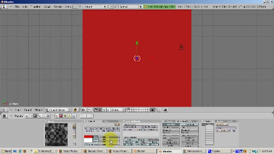
Position the camera directly at the plane with View - Align View - Align Active Camera to View.

Go to Front View (Num1). Press the Home key to see all the objects, particularly, the camera. Duplicate the plane (Shift-D). Move the plane upwards, in the Z direction (press the G key and then the Z key), so that it is behind the camera. The duplicated plane has Ray Mirror on as well.

Go to the Scene buttons (F10). Make sure the Ray button is turned on, so that Ray Tracing is enabled.



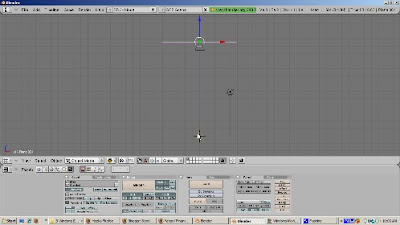
Center the 3D cursor by pressing Shift-C. Add the monkey (Space - Add - Mesh - Monkey). Add a new material by pressing F5 (Shaders) and clicking the Add New button. Make Suzanne green (R=0, G=1, B=0). Move the monkey 1 blender unit to the right and up a bit. Go to Edit buttons (F9). Press the Set Smooth button. Add a Subsurf Level 2, Render Level 3.

Make sure you are in Object Mode. If not, press the tab key. Add a UV Sphere (Space - Add - Mesh - UVSphere). Give the UV Sphere a blue color by going to the Shaders panel (F5), adding a new material (Add New button) and setting R=0, G=0, and B=1. Move the UV Sphere 2 blender units to the left and up a bit, off the floor of the plane. Press F9 to go to the Edit buttons. Click the Set Smooth button to smooth out the UV Sphere.

Press F12 to render. The red mirror should show the mirroring of both the monkey and the UV Sphere, as the light bounces off the bottom mirror, sees the monkey and the UV Sphere, and then the objects are mirrored off the top mirror. The shadow obscures somewhat the mirrored effect.



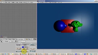
Let's turn off shadows. Go to the Scene buttons (F10) and click off Shadow. Press F12 to render. Now you get the effect of both the top mirror and the bottom mirror.




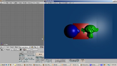
The mirror effect can be combined with the color effect. Select either mirror plane (Right click). Press F5 to access the Shaders buttons. In the Ray Mirror group, turn Ray Mirror to 0. Press F12 to render. There is no mirror effect. The monkey and the UV Sphere both render, and the plane is red.



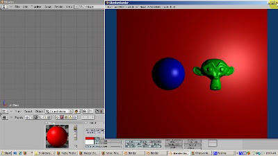
Now set Ray Mirror to .5, so we get half mirror and half color. Press F12 to render. Now the red base color shows through, but the mirror effect shows through as well. You can play with Ray Mirror to get the combination you like.



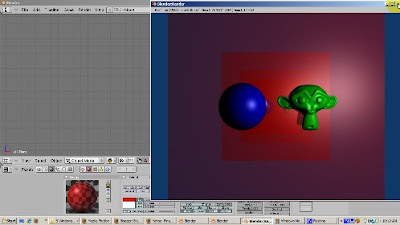
The mirror color can also play a role. Turn Ray Mirror back to 1 so we get the full ray mirror effect. Now let's set the mirror color to yellow. Select the Mirror color rectangle, and change it to Yellow (R=1, G=1, B=0). Press F12 to render. We get a really interestng result. The yellow mirror color mixes with the material's color. The monkey is green. Yellow already has green. So the mirrored monkey remains green. However, the sphere is blue. The mirror color, yellow, has no blue, so the mirrored UV sphere is yellow. By the way, there's also a blending with the sky color, which is also mirrored, which accounts for the color variation outside the mirror boundary.



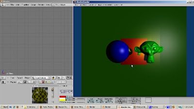
The Depth setting controls how many times the mirror effect bouncing is produced. Let's crank up the depth to 5 and press F12 to render. There are now more mirrored monkeys and UV Spheres.



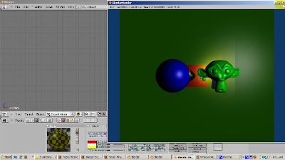
The Fresnel setting produces another interesting effect, mixing the mirror color, and the mirror's diffuse color. Let's crank Fresnel to 1.5 and render.



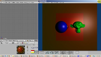
The Glossiness setting affects the blurriness of the reflection. The default of 100% glossiness produces a crisp reflection. A little bit of reduction goes a long way in increasing the realism of the render. Set glossiness to .9 (90%) and you'll get an effect that simulates a bit of dirt in the mirror.



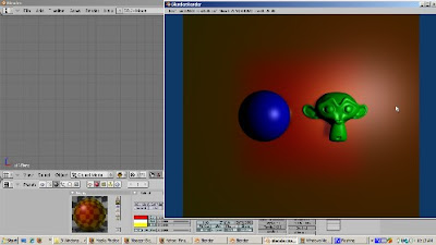
There's more. How about turning on Ray Mirror for the monkey and the UV Sphere. Select the monkey. Go to the Shading buttons (F5). Click the Ray Mirror button. Turn RayMir to 1. Then select the UVSphere, go to the shading buttons, and turn on Ray Mirror, setting it to 1. Press F12 to render. How about changing the mirror's shape? Subdivide the plane, rotate a few vertices, and render. I'll leave that to you.




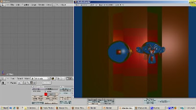
As you can see, there are a lot of neat effects you can achieve with Ray Mirror. I hope you have the basis for experimenting more and getting the effect you desire. Happy Blendering!

Multiple Materials

Join my Blender 3D forum, where you can network with other Blender friends and get your Blender 3D questions answered.



Many times you will be assigning one material to an entire object. However, there are situations where you want to assign different parts of an object to their own material. The assignment can get kind of tricky. In this demo, we will make each face of a cube have a different colored material. You can then extend this to customize each material, such as changing its opacity or transparency, on each face. You can also add separate textures to each material. This tutorial shows you how to do the first step: creating a separate material for each face of a cube.

Steps:
1) We'll start with the default 2.49b scene and use the default cube. Press Tab to go to Edit mode. Go to Face Select mode (Control - Tab - 3 or the triangle icon. Press A to deselect all faces. Rotate the cube on its side, to make selecting a face easier. Press Z to go to wireframe mode.

Materials are assigned per face. Each face can have only 1 material ID. New materials are given the next material ID, 2 for the second one, 3 for the third one, and so on. A set of buttons in Edit (F9( assigns multiple material IDs. By default, when you Add New material, all faces have a Material ID 1. Press F5 for the shading buttons. There's an indicator (1 Mat 1) that shows how many materials are on the object (1), and which one we're working on (1).

2) Create 5 new materials. By default, each face of the cube has a material, called Material, assigned to it. The Material button group shows that there is 1 material assigned to the cube. Press F9 to get to the Editing buttons. Press the New key 5 times. Now there are 6 materials, with the names Material, Material.001, Material.002, all the way to Material.005.

3) Assign the faces to their respective materials:
Go to F9 (Editing buttons). Assign the faces as follows:
Select the top face. Set its material to Material (ID = 1). Click Assign.
Select the bottom face. Set its material to Material.001 (ID = 2). Click Assign.
Select the left face. Set its material to Material.002 (ID = 3) Click Assign.
Select the right face. Set its material to Material.003 (ID=4). Click Assign.
Select the front face. Set its material to Material.004 (ID = 5). Click Assign.
Select the back face. Set its material to Material.005 (ID=6). Click Assign.

You can verify which material is associated with which face. Press the A key to deselect all faces. Select a material, say Material.004. Click the Select button and you should see that the material is assigned to the top face. You can also do the opposite. Press A to deselect all faces. Click the bottom face. Click the question mark icon. You should see that Material.001, with material ID 2, is assigned.

4) Click F5 to go to the Shading buttons. We want our materials to have meaningful names so we can identify them easily. Assign the following colors:
Material: Red (R=1, G=0, B=0). Press Autoname to have Blender create a meaningful name (Red).
Material.001: Green (R=0, G=1, B=0). Press Autoname. Blender calls this LightGreen.
Material.002: Blue (R=0, G=0, B=1). Press Autoname. Blender calls this LightBlue.
Material.003: Yellow (R=1, G=1, B=0). Press Autoname. Blender calls this material Yellow.
Material.004: Magenta (R=1, G=0, B=1). Press Autoname. Blender calls this material Magenta.
Material.005: Cyan (R=0, G=1, B=1). Press Autoname. Blender calls this material Cyan.

To view our result, press Tab to go into Object mode. Then go into Shaded mode. Rotate the cube. Press F12 to render.

You can further refine this by changing the characteristics of a material by playing with settings such as Ray Mirror, Alpha, Ray Transparency, the render pipeline, and so on. You can produce some interesting effects. Happy Blendering.

Rip Tool

Join my Blender 3D forum, where you can network with other Blender friends and get your Blender 3D questions answered.



The Rip tool lets you tear out a hole, such as a mouth or an eye socket if you're modeling a face, in your mesh. You can use the Rip Tool in either vertex select or edge select mode. The Rip Tool does not work in Face Select Mode. You can also use the Rip tool to do split apart a mesh, for example, splitting a sphere into two halves. You can create faces to join the parts of the mesh that you have ripped. The goal of this tutorial is to make you comfortable both ripping a mesh apart to create holes where you want them, and to join mesh parts together again.

We'll start with the default Blender 2.49b scene. Delete the default cube (press the Delete key and press Enter to confirm). Add a plane (Space - Add - Mesh - Plane). The plane is in Object mmode. Scale the plane to 4 times its original size (S - 4 - Enter). Get rid of the 3D Transform Manipulator to make the demonstration of the Rip Tool easier to follow.

Press Tab to go into Edit mode. Press the Edit buttons (F9) and click the Subdivide button 3 times. Press the A key to deselect all vertices.

Look at the indicators for vertices, edges, and faces. Right now, the plane has 81 vertices, 144 edges, and 64 faces. The zeroes show that nothing is selected.

Make sure you are in Vertex Select Mode (Control - Tab - 1) or the Vertex Select icon. Position the 3D cursor below and to the right of the vertex you want to select. Select the vertex, then press the V key, grabbing the vertex to the right. A hole is created to the right of the vertex. Look at the indicators for vertices, edges, and faces. Before the plane had 81 vertices, of which none were selected. Now, the plane has 82 vertices, and one is selected.

This gives a clue as to what the Rip tool actually does. It creates a duplicate vertex at the same spot as the selected vertex, connected to the vertices as the copied vertex. When the mesh is ripped, that vertex drags the adjacent edges with it. The 3D cursor position determines the direction of the rip.

Press Alt-U, which brings up the Undo History. Click on Select to undo the rip. Now we're back to having the vertex selected, with 81 vertices altgether. Move the cursor above and to the left of the selected vertex. You can constrain the rip to an axis. To do that, press the V key, and then the Y key to constrain the rip to the Y axis. Press Enter to confirm. So you can see that the direction of the rip depends on the position of the 3D cursor at the time that you press the V key. The rip is along the edge that is closest to the selected vertex.

Press the A key to deselect the vertex. Go to another part of the plane, and select a vertex. Then Shift select (Shift - Right Click) the vertex immediately to the right of it. Position the 3D cursor above and in the middle of the selected vertices. Press the V key. You now get a bigger rip, a trapezoid, with 2 vertices on top and 4 vertices on the bottom. So a rip with N selected vertices produces a ripped polygon with N vertices in the ripped direction and N+2 vertices in the original direction.

If you start the Rip and then immediately decide not to continue, the new vertices still remain. To illustrate this, select a vertex, press the V key, and then press Esc. The vertex created by the Rip tool is still there. You can rip the mesh now even though you pressed Esc. Press the G key and move the vertex and the mesh is ripped. Press Enter to confirm.

Press the A key to deselect all vertices. Suppose you want to patch up the hole that you created. The solution is to select the vertices for the new face (3 or 4) and press the F key. To illustrate this, select the 4 vertices that form the square of the hole created from 2 selected vertices. Press the F key. A face is created.

Press the A key to deselect all vertices. Now we'll create triangular faces for the remaining two holes. Select the 3 vertices forming the left triangle, and press F. Press the A key to deselect everything. Select the 3 vertices forming the right triangle, and press F. The hole is now repaired. Press the A key to deselect.

Ripping via an edge loop is a great way to split a mesh. Select an Edge Loop by positioning the 3D cursor on an edge and pressing Alt-Right Click. Then press the V key and scroll down. Press Enter to confirm. You have now split the mesh along the edge loop.

Rip works in edge mode as well. Go into Edge mode, by either selecting the Edge icon or pressing Control - Tab - 2. Position the 3D cursor above an edge to select. Select the edge (Right Click on an edge). Press the V key. The rip works just like selecting two adjacent vertices, which is, of course, what constitutes an edge.

Press the A key to deselect everything. You rip on two edges along the same loop. Select an unselected edge. Then Shift Select (right click while holding the Shift key) to select the edge next to it. Press the V key. The rip works in the trapezoidal fashion you would expect.

Rip works on other meshes as well. Let's look at a UV Sphere. Press tab to go to object mode. Click the second square to go to Level 2, so we have a blank 3D viewport. Add a UV Sphere (Space - Add - Mesh -UVSphere), accepting the default of 32 rings and 32 segments. Press Z to go into wireframe mode. Scale the UVSphere 3 times (S - 3 - Enter). Press Tab to go into Edit mode. Go into Edge select mode (Control - Tab - 2). Press the A key to deselect everything.

Press Num 1 key to go to front view. Position the cursor on an edge and press Alt-Right Click to select an edge loop. Position the 3D cursor below the selected loop. Press the V key. Move the selected edge loop down. Behold, you have split the UV Sphere. Press Z to go into solid mode so you can see.

Ycu can also rip and scale at the same time. Select another edge loop (Alt- Right Click) for splitting the UV Sphere. Position the 3D cursor below the loop. Press the V key, then the Z key to constrain along the Z axis, drag the edge down. Press Enter. Then press the S key to scale the loop.

I hope this gives you a good idea of the Rip tool, which is very handy for creating holes in a mesh. Happy Blendering!

2.49b Edge and Face Loops

Join my Blender 3D forum, where you can network with other Blender friends and get your Blender 3D questions answered.



You can select the subcomponents of a mesh by either right clicking, or shift right click, or the B key to box select, or the B key twice to form a circle selection, or alt left click for lasso select. There's another way to select parts of a mesh, which is by selecting a loop of vertices, edges, or faces. Also, adding loops is a great way to add detail to your mesh. Instead of subdividing a mesh, which adds a lot of extra geometry when it's not needed, adding loops only in the area where you want detail will create a cleaner mesh with fewer edges, vertices, and faces. The aim of this tutorial is to demonstrate how to use loops both to select parts of your mesh and to add details to it.

Selecting By Loops

We'll work with the default cube. It's selected and in Object Mode. Go to the Edit buttons (F9) and press Tab to go into Edit mode. Press the Subdivide button, in the Mesh Tools panel, three times. Rotate the view, using either the middle mouse button or alt-Left Mouse Button if you enabled Emulate 3 Button Mouse in the Preferences window. We're in Vertex Select mode. Position the 3D Cursor at one of the corner vertices. Hold the Alt key down and press the Right Mouse button. Doing that, selects not just the vertex (which is what Right Mouse button does just by itself), but the entire edge that the vertex belongs to.



Press the A key to deselect the vertices.

Now hold the Alt key down and select a vertex that is not on the outside edge but instead is inside the cube. This time, an entire loop of edges is selected - the loop that that vertex belongs to. The loop could be horizontal or vertical.



Press the A key to deselect everything. You can also select the perpendicular range of faces to which the edge belongs by holding both the Control key and the Alt key at the same time. To illustrate, press the Control key and the Alt key at the same time, and select a vertex. What is selected is the faces on the edge perpendicular to the vertex.



You can add to the loop selection, in effect selecting multiple loops, by holding the Shift Key down as well as the Alt Key. Hold the both the Alt and Shift keys and select an unselected vertex. Now you have selected two loops. If the loop includes all the vertices that form a face, those faces will be selected as well.



If you feel particularly ambidexterous, try holding the Control, Alt, and Shift keys down at the same time, and select another vertex. You then add to the faces selected before.

Loop selection works in edge select mode as well. Holding the Alt key and then clicking the right mouse button selects the loop to which the edge belongs to. Press the A key to deselect everything. If we go into Face Select mode, we see that loops of faces can also be selected this way. Hold the Alt kay, and with the 3D cursor on a face, press the right mouse button to select a face loop. Hold both the Shift key and the Alt key, select an unselected face with the right mouse button, and the loop in which the selected face belongs is added to the selection.



Selecting loops of vertices, edges, or faces, can make the selection process much more precise than box selection or selection of individual vertices, edges, or faces.

Creating Loops On A Cube

You can add edge loops with the Loop Subdivide tool (Control-R). To illustrate, position the cursor on an edge of the cube, and press Control-R. A magenta square shows where the new loop will be cut. However, you actually have more control over where the loop cut will occur. Press Enter.



Now you see both the proposed new loop, and a green line, which is the edge along which you can slide this loop. This is called "edge slide mode". A green line, showing the edge along which the loop can be cut, displays. You can scroll the edge up and down along the green line. Press Enter when you get to the position of the new edge that you want.

You can create more than one edge loop at a time. Position the cursor at an edge along where you would like to cut and press Control-R. Now, instead of pressing Enter, press the + key on the numeric keypad. This adds a loop cut, allowing you to create two loop cuts at a time. You can press the + key on the numeric keypad to add another loop cut, or you can press the - key on the numeric keypad to subtract 1 loop cut. Then press Enter. Edge Slide mode does not work when you create more than one edge loop. Instead, the loops are split evenly along the edge.



Creating Loops On A UV Sphere

Let's start with the default scene by selecting Load Factory Settings from the menu. Delete the default cube (press the Delete key, then press OK to accept the delete). Add a UV Sphere (Space - Add - Mesh - UVSphere), accepting the default settings of 32 rings and 32 segments. Press Tab to go into Edit Mode. Press A to deselect everything. Press Control-R. You can create edge loops either based on rings (going left and right) or segments (going up and down). Lets add an edge loop based on a ring. Press Control-R, selecting a horizontal edge loop to create. This selection works the same way as for a cube. Press Enter, to go into Edge Slide mode. Position the loop where you want and press Enter. However, for a ring, the edge loop only is created on half the UV Sphere. Press Control-R, then Enter. Slide the edge where you want it. Then press Enter. Rotate the UV Sphere and you will see the result. To get the edge loop to go around the UV Sphere, you will need to create the corresponding edge loop on the other side of the sphere.




You can add more than one loop cut using the + key on the numeric keypad, and subtract using the - key on the numeric keypad, as with the cube.

Control - Alt - Right Click and Shift - Control- Alt - Right Click work the same way on a UV Sphere as on a cube. You can create a loop of faces perpendicular to the edge you select with Control - Alt Right Click, and extend the selection if you somehow manage to hold Shift, Control, Alt, and Right Click while the 3D cursor is on an unselected face.

As you can see, selecting and adding loops can make your mesh modeling more precise when you're adding detail. These techniques work on any mesh, not just the cube or UV Sphere. Try them with a torus, or with Suzanne, and you should get the hang of loop selection and addition quickly. Happy Blendering!

Incredible Machines Book

There's an exciting book coming out soon, called Blender 3D 2.49 Incredible Machines. The video shows an example of what the reader will be able to create, using Blender 3D to model the entire scene and setup all lights and materials with LuxRender. In LuxRender we will use an incredible feature called Light Groups to control all lights on the scene, with the image still rendering. Notice that we can turn on and off all lights and see the result in real time, and there are lots of other possible adjustments like the temperature of light and much more.

The video is based on the book's third project. It was created by the author, Allan Brito. Allan is an active member of the Blender development community. He's a Brazilian architect who specializes in information visualization. This is his 3rd Blender book.

This book will show you how to use Blender 3D for mechanical modeling and product visualization. Through the pages of the book, you will find a step-by-step guide to create three different projects: a fantasy weapon, a spacecraft, and a giant robot. Even though these machines are not realistic, you will be able to build your own sensible and incredible machines with the techniques that you will learn in this book along with the exercises and examples.

If you want to model machines and want to understand in depth industrial uses of Blender, this sounds like a book to examine closely.

2.50 Alpha 0 Tools Menu

Join my Blender 3D forum, where you can network with other Blender friends and get your Blender 3D questions answered.



November 24, 2009 marks a milestone for all Blender users because it is the release date of Blender 2.5 Alpha 0. While there is still much work to do, the release of Alpha 0 means that Blender 2.5 is formally open for user comments, testing, and feedback, at Blender Foundation's blender.org site.

You can download Alpha 0 from Blender.org.

You should also read the Alpha 0 Release Notes. These give us a much clearer path of where Blender 2.5 is headed.

Some time ago, I did a Blender 2.5 Sneak Preview Video, based on a pre-alpha version of 2.5. Although much of what I discussed is still valid, Blender 2.5 has evolved since then. Also, my understanding of certain features is clearer now than it was 2 months ago. So I thought it would be a good time to revisit, highlighting the new ways of doing things. This tutorial focuses on a particularly interesting new feature, the Tool Shelf, which reorganizes access to Blender tools into one menu.



Before we start on the Tool Menu, note that the Startup Screen has a window with links to places where we can get the latest information about Blender 2.5 - the Release Log, the Manual, the Blender.org Web site, the user community, and the Python API reference. For example, clicking the Manual link opens up a browser window with the Blender 2.5 manual, which is a wiki. I encourage you to check these links out because Blender 2.5 is developing rapidly and you don't want to miss out on the newest goodies.

You get rid of this initial splash screen by left clicking on it. In Blender 2.5, the default scene still consists of the cube, camera, and lamp objects. The Tool Menu, what we're going to focus on, is the menu at the left side.



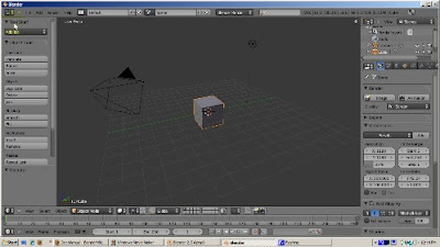
There are actually three sections to the menu. The top most section, the Tool Shelf, initially contains no tools. Its purpose is to give you the flexibility of adding your favorite tools, available from the click of a button. You can add a tool by clicking the Add Tool button. A list of tools displays. You can select one of those, but actually the best way to add a tool is to search for it. Let's suppose you want to save your .blend file frequently and want a button to do that. Instead of scrolling down the list of choices - there are a lot of them because it's all the possible things you can do in Blender - go to the search box (the box with the magnifying glass icon), and type the word Save. You get a list of all the Blender tools with the word Save in it. Choose Save Blender File. Now you can save the file with the click of a button. You can add as many buttons as you want to the Tool Shelf. Maybe you also append objects from libraries often. You can add the Link/Append From Library button. You can easily customize the Tool Shelf to include all the things you do in Blender frequently, without having to wade through a maze of buttons, and panels.



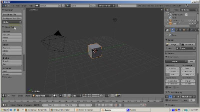
The next group of tool menus actually changes depending on what mode you are in. Blender starts up, as it did before, with the default cube selected and in Object Mode. Since Object Mode is selected, the tools available in Object Mode, such as Translate, Rotating, and Scaling, Smoothing, and Inserting Keyframes, display. To show how these choices change, press the Tab key to go into Edit Mode. Note that the indicator shows that edit mode is active. The tools that are applicable to meshes, such as Extrude, Subdivide, Loop Cut, as well as Translate, Rotate, and Scale, now display.

Click Tab again to go back to Object Mode. Note that the Object tools are available again. To demonstrate the bottom part of the Tool Menu, let's scale the cube up, to 3 times its original size. We're going to try to do it through the GUI but will not be successful. What would have happened in Blender 2.4x is that you would have to bring up the Transform Properties menu and change the size. This means you would have had to know about that menu. In 2.5, the options for Resize automatically display at the bottom of the Tool Menu. You can resize by changing the values there. Also, you can scroll down to get all the options available when resizing.

Now let's duplicate the cube. Press the Duplicate key. Just like Shift-D, which still works, the cube is duplicated. Move the new cube away from the old cube to see. Note that the bottom right part of the Tool Menu changed to show the options for duplicating an object. By changing the options, say to make a linked duplicate, you chane how Duplicate works. This gives you immediate visual feedback.

Another neat feature is Repeat Last. Click on Repeat Last. The last operation - in this case the duplication - is repeated. Move the new cube away from the old cube and you can see it. Repeat Last works for most operations. If you're doing some operation, like extruding or scaling, or creating edge loops, a number of times, you can save a lot of time by clicking on Repeat Last.

You can see the tools available in other modes by switching mode. Sculpt Mode, for example, shows the various brushes and settings for each type of sculpting. Weight Paint shows the Weight Paint tools. Vertex Paint shows the vertex paint tools, and so on. The specific options for each tool are on the Tool Menu, at your fingertips. This should help make your workflow more efficient.



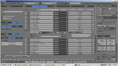
Another powerful addition in 2.5 is that the shortcuts are totally configurable. Go to the User Preferences and select the Input panel, which is selected by default. If you wanted Save File to be something other than Ctrl-W, first click the Edit button to make the keys editable. Then, find where Save File is stored. Expand the choice by clicking on the left arrow. You can change the keypress to something else, say, Control-Shift-W. You can do this for other functions. If you want these changes to be permanent, click the Save As Default button. Otherwise, the changes will be lost when you exit Blender. You can also save your key maps. The idea is that, if you use another modeling package, such as Maya, you can map the operations you used there into Blender.

I hope this gives you a taste of the new Tool Menu in Blender 2.5 alpha 0. Although everything is subject to change, something this fundamental is likely to be around when Blender 2.5 is finally released into production.

2.49b Vector Blur

Vector blur is a great way to add realism to your animation. Your eye naturally sees moving objects moving as a blur, because that is how your brain processes the motion. Without some sort of blurring, animated moving objects don't look as if they are realistically moving. Blender's animations are by default rendered as a sequence of perfectly still images. This is unrealistic, since fast moving objects do appear to be 'moving', that is, blurred by their own motion, both in a movie frame and in a photograph from a 'real world camera'.

To obtain such a blurring effect with moving objects, Blender can be made to render the current frame and some more frames, in between the real frames, and merge them all together to obtain an image where fast moving details are 'blurred'. The goal of this tutorial is to demonstrate how to blur moving objects in Blender.

First, we'll create a simple animation. We will animate the movement of the cube across the screen, over 50 frames. With an animation speed of 25 frames per second, that produces a 2 second video, one second going across the screen, the other second going back.

1) Go to the SR-1: Animation view.
2) Press the N key to bring up the Transform Properties window. Set the X location to -7, the Y location to 0, and the Z location to 0.
3) At Frame 1, press the I key and insert a Location key frame.
4) Go to Frame 25. Set the X location to 4, the Y location to 0, and the Z location to 0.
5) Press the I key and insert a Location key frame.
6) Go to Frame 50. Set the X location to -7, the Y location to 0, and the Z location to 0.
7) Press the I key and insert a Location key frame.

8) Go to the Scene buttons (F10), and set the animation to 50 frames.
9) In the Format panel, set the animation type to your favorite. I used the compressed AVI format with the CamStudio Lossless Codec, version 1.4, for compression.
The video will be created in the Output directory (/tmp by default), with a filename of 0001_0050.avi. Set the output directory to the folder where you want the video to be saved. If you chose a QuickTime movie, the filename would be 0001_0050.mov.

10) Hit the ANIM button. I will pause the video while the animation is being rendered, as I will do for the other animations in this video. The render took 1 minute, 10 seconds.

The animation does indeed have the cube move back and forth, but the motion of the cube is not realistic. The cube just moves in a straight line uniformly, without the blurring effect of motion.

With the help of the Node editor, we can introduce vector blur to this animation and compare. To do this,

1) Go to the Render Layers tab of the Scene button. Vector blur takes a special Vector (VEC) rendering pass, which is not rendered by default. Find the VEC button and enable it. Vector Blur requires the COMBINED, Z, and VEC passes. The others you may need to render the scene exactly as you need it.

2) Change the 3D view to the Node Editor. Press Control-Down Arrow to maximize te Node Editor. Click on the face, for composite nodes. Then click the USE NODES button. There are two default nodes, the input node (Render Layers) is the scene as rendered without compositing. The other node, the Composite node, is the final result of the compositing process.

3) Move the Composite Node all the way to the right, to make room for the Vector Blur.

4) Add the Vector Blur filter (Space - Add - Filter - Vector Blur). Accept the defaults. Connect the Image socket of the Render Layer to the Image input of the Vector Blur node. Connect the Z socket of the Render Layer node to the Z socket of the Vector Blur node. The Z socket stores the Z information - the distance of the cube from the camera. Connect the Speed socket of the Render Layer node to the Speed socket of the Vector Blur node. The Speed socket is really the key to blurring the cube's movement. You can play with the defaults. Increasing the number of samples, for example, makes the vector blur more realistic but slows down the rendering. Also, you can control which moving objects are blurred. A speeding sports car should be blurred, but bystanders should not.

5) Connect the Image output socket of the Vector Blur node with the Image socket of the Composite node.

The noodle (the node setup) is complete. Go back to the Scene buttons and click the Do Composite button. Press the Render button. Look at Frame 1. The monkey is blurred.

6) Time to animate. Click the ANIM button. Pause until the 50 frames are rendered. The render took 1 minute, 47 seconds.
Now you see the cube blurred while it is moving --- a much more realistic animation. Think of a fast sports car speeding by you.

Blender has another way to implement blurring a moving object: the Motion Blur option. To demonstrate that, click the MBLUR button in the Scene panel. Turn off Do Composite because motion blur doesn't rely on nodes. MBLUR is very slow because it renders each frame up to 16 times. The number of samples is controlled by the OSA setting, which is 8 on my computer. Eight renders per frame is mighty slow. The renderer calculates the position of each object and then averages the positions out. It is more accurate than Vector Blur, but at the cost of a LOT of time. Here is the cube animation with motion blur.

To summarize, Blender provides you with two options, Vector Blur and Motion Blur, for making your moving object look more realistically blurred as the object moves in the scene. For most applications, especially in the Game Engine, Vector Blur will work well. Happy Blendering!